AKDE: Multivariate Adaptive Kernel Density Estimation Using Gaussian Mixture Model

AKDE provides a accurate, adaptive kernel density estimator based on the Gaussian Mixture Model for multidimensional data. This Python implementation includes automatic grid construction for arbitrary dimensions and provides a detailed explanation of the method.

Installation

pip install akde

Usage

from akde import akde
pdf, meshgrids, bandwidth = akde(X, ng=None, grid=None, gam=None)

Function Descriptions

akde(X, ng=None, grid=None, gam=None)

Performs adaptive kernel density estimation on dataset X.

• X: Input data, shape (n, d), where n is the number of samples and d is the number of dimensions.
• ng (optional): Number of grid points per dimension (default grid size based on dimension d).
• grid (optional): Custom grid points for density estimation.
• gam (optional): Number of Gaussian mixture components. A cost-accuracy tradeoff parameter, where gam < n. The default value is gam = min(gam or int(np.ceil(n ** 0.5)), n - 1). Larger values may improve accuracy but always decrease speed. To accelerate the computation, reduce the value of gam.

Returns:

• pdf: Estimated density values on the structured coordinate grid of meshgrids (shape: (ng ** d,)). To reshape pdf back to match the original structured grid for visualization:

   pdf = pdf.reshape((ng,) * d)

• meshgrids: Grid coordinates for pdf estimation (A list of d arrays, each of shape (ng,) * d)
• bandwidth: Estimated optimal kernel bandwidth (shape (d,))

EXAMPLES

1D data

import numpy as np
import matplotlib.pyplot as plt
from scipy.stats import norm
from akde import akde

# Set random seed for reproducibility
np.random.seed(42)
n_samples = 1000

# Define 5 Gaussian mixture components (means, standard deviations, and weights)
means = [-4, -2, 0, 2, 4]       # Different means
stds = [0.5, 0.8, 0.3, 0.7, 1.0]  # Different standard deviations
weights = [0.2, 0.15, 0.25, 0.2, 0.2]  # Different weights (sum to 1)

# Generate samples from each Gaussian distribution
data = np.hstack([
    np.random.normal(mean, std, int(n_samples * weight))
    for mean, std, weight in zip(means, stds, weights)
]).reshape(-1, 1)  # Reshape to (n,1) for AKDE

# Perform adaptive kernel density estimation
pdf, meshgrids, bandwidth = akde(data)

# Reshape the PDF to match the shape of the grid
pdf = pdf.reshape(meshgrids[0].shape)

# Compute the true density function by summing individual Gaussians
true_pdf = np.sum([
    weight * norm.pdf(meshgrids[0], mean, std)
    for mean, std, weight in zip(means, stds, weights)
], axis=0)

# Plot the density estimation, true distribution, and histogram
plt.figure(figsize=(8, 5))
plt.hist(data, bins=50, density=True, alpha=0.3, color='gray', label="Histogram (normalized)")
plt.plot(meshgrids[0], pdf, label="AKDE", color='blue', linewidth=2)
plt.plot(meshgrids[0], true_pdf, label="True Distribution", color='red', linestyle='dashed', linewidth=2)
plt.xlabel("X")
plt.ylabel("Density")
plt.title("Histogram vs AKDE vs True Distribution")
plt.legend()
plt.savefig("1D-AKDE-Density.png", transparent=False, dpi=600, bbox_inches="tight")
plt.show()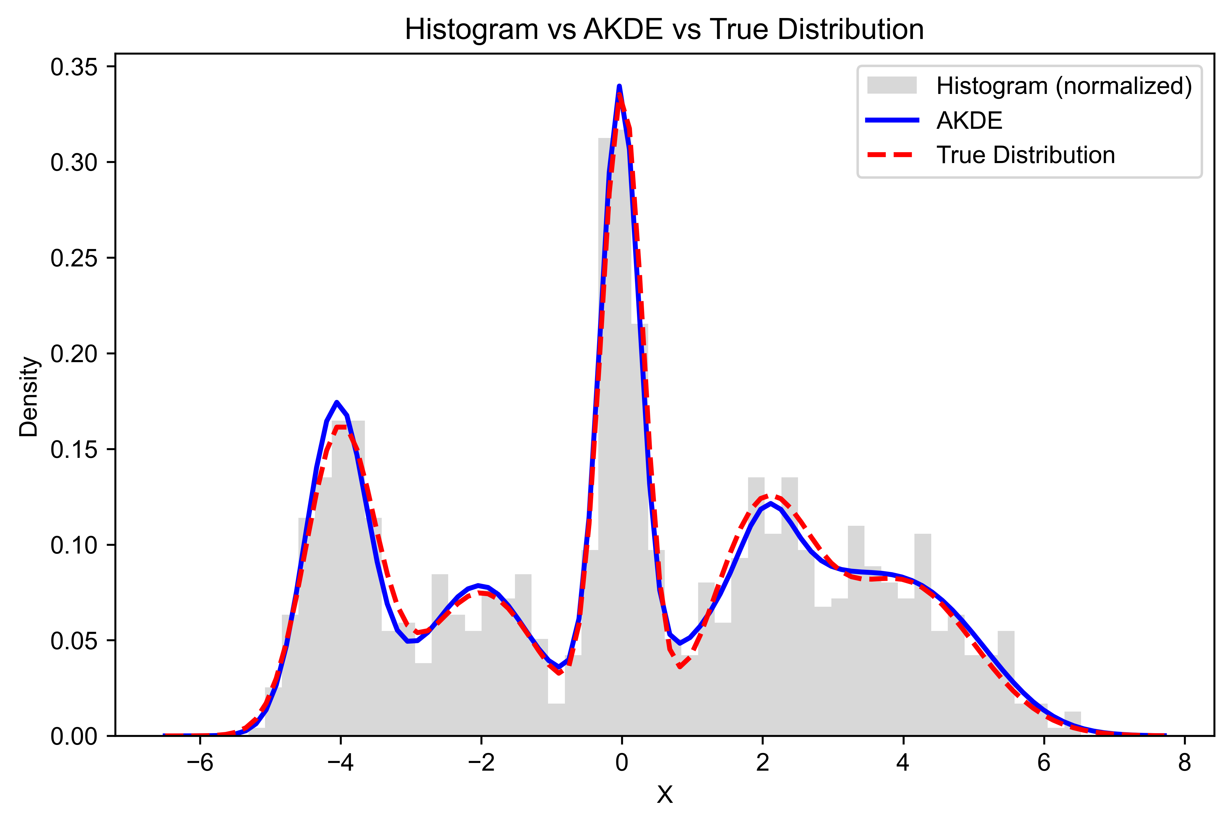

2D data

import numpy as np
import matplotlib.pyplot as plt
from akde import akde

# Generate synthetic 2D mixture distribution data
np.random.seed(42)
n_samples = 1000

# Define mixture components
mean1, cov1 = [2, 2], [[0.5, 0.2], [0.2, 0.3]]
mean2, cov2 = [-2, -2], [[0.6, -0.2], [-0.2, 0.4]]
mean3, cov3 = [2, -2], [[0.4, 0], [0, 0.4]]

# Sample from Gaussian distributions
data1 = np.random.multivariate_normal(mean1, cov1, n_samples // 3)
data2 = np.random.multivariate_normal(mean2, cov2, n_samples // 3)
data3 = np.random.multivariate_normal(mean3, cov3, n_samples // 3)

# Combine data into a single dataset
X = np.vstack([data1, data2, data3])

# Perform adaptive kernel density estimation
pdf, meshgrids, bandwidth = akde(X)

# Reshape the PDF to match the shape of the grid
pdf = pdf.reshape(meshgrids[0].shape)

# Plot the density estimate
plt.figure(figsize=(8, 6))
plt.imshow(pdf, extent=[meshgrids[0].min(), meshgrids[0].max(),
                        meshgrids[1].min(), meshgrids[1].max()],
           origin='lower', cmap='turbo', aspect='auto')

plt.colorbar(label="Density")
plt.scatter(X[:, 0], X[:, 1], s=5, color='white', alpha=0.3, label="Data points")
plt.xlabel("X")
plt.ylabel("Y")
plt.title("2D DATA DENSITY PLOT")
plt.legend()
plt.savefig("2D-AKDE-Density.png", transparent=False, dpi=600, bbox_inches="tight")
plt.show()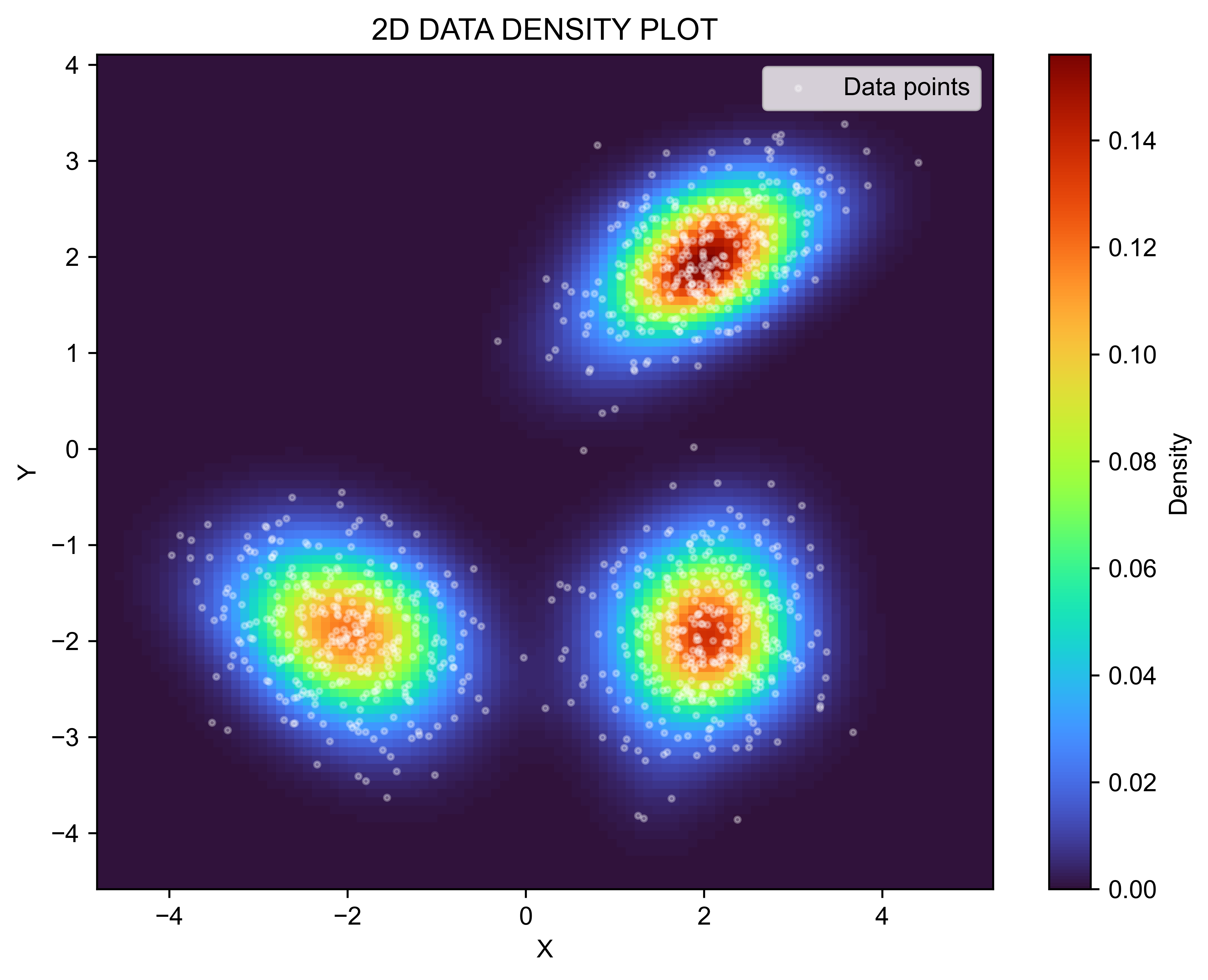

2D data Density plot using matplotlib imshow function

3D projection plot of the same 2D data Density using Plotly Surface

import numpy as np
import plotly.graph_objects as go
from akde import akde

# Generate synthetic 2D mixture distribution data
np.random.seed(42)
n_samples = 10000

# Define mixture components
mean1, cov1 = [2, 2], [[0.5, 0.2], [0.2, 0.3]]
mean2, cov2 = [-2, -2], [[0.6, -0.2], [-0.2, 0.4]]
mean3, cov3 = [2, -2], [[0.4, 0], [0, 0.4]]

# Sample from Gaussian distributions
data1 = np.random.multivariate_normal(mean1, cov1, n_samples // 3)
data2 = np.random.multivariate_normal(mean2, cov2, n_samples // 3)
data3 = np.random.multivariate_normal(mean3, cov3, n_samples // 3)

# Combine data into a single dataset
X = np.vstack([data1, data2, data3])

# AKDE
pdf, meshgrids, bandwidth = akde(X)

Z = pdf.reshape(meshgrids[0].shape)

fig = go.Figure(data=[
    go.Surface(
        x=meshgrids[0], y=meshgrids[1], z=Z,
        colorscale='Turbo',
        opacity=1,
        colorbar=dict(
            title="Density",
            titleside="right",
            titlefont=dict(size=14),
            thickness=15,
            len=0.6, 
            x=0.7,  
            y=0.5
        )
    )
])

# Update layout settings
fig.update_layout(
    title="",
    scene=dict(
        xaxis_title='X',
        yaxis_title='Y',
        zaxis_title="Density",
        xaxis=dict(tickmode='array', tickvals=np.arange(-10, 11, 2.0), showgrid=False),
        yaxis=dict(tickmode='array', tickvals=np.arange(-10, 11, 2.0), showgrid=False),
        zaxis=dict(tickmode='array', tickvals=np.arange(0, 0.6, 0.1), showgrid=False), 
    ),
    margin=dict(l=0, r=0, t=0, b=0)
)

fig.update_layout(scene = dict(
                    xaxis = dict(
                         backgroundcolor="rgb(255, 255, 255)",
                         gridcolor="white",
                         showbackground=True,
                         zerolinecolor="white",),
                    yaxis = dict(
                        backgroundcolor="rgb(255, 255,255)",
                        gridcolor="white",
                        showbackground=True,
                        zerolinecolor="white"),
                    zaxis = dict(
                        backgroundcolor="rgb(255, 255,255)",
                        gridcolor="white",
                        showbackground=True,
                        zerolinecolor="white",),)
                  )
  
fig.update_scenes(xaxis_visible=True, yaxis_visible=True,zaxis_visible=False)
fig.update_layout(paper_bgcolor="rgba(0,0,0,0)", plot_bgcolor="rgba(0,0,0,0)", autosize=True)
fig.write_html("2D-AKDE-density-3D-projection.html")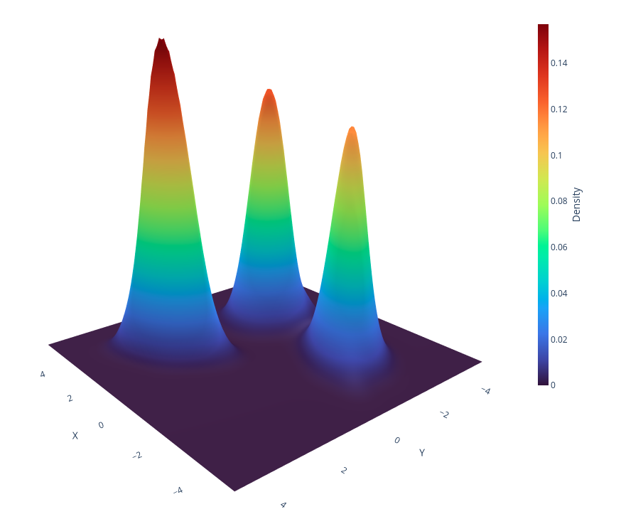

3D data

import numpy as np
import plotly.graph_objects as go
from akde import akde

# Set random seed for reproducibility
np.random.seed(12345)

# Number of samples
NUM = 10000

# Generate synthetic 3D data (mixture of 3 Gaussians)
means = [(2, 3, 1), (7, 7, 4), (3, 9, 8)]
std_devs = [(1.2, 0.8, 1.0), (1.5, 1.2, 1.3), (1.0, 1.5, 0.9)]
num_per_cluster = NUM // len(means)

# Create 2D numpy array data with shape: (NUM, 3)
data = np.vstack([
    np.random.multivariate_normal(mean, np.diag(std), num_per_cluster)
    for mean, std in zip(means, std_devs)
])  

# AKDE 
pdf, meshgrids, bandwidth = akde(data) 

# ====== PLOTTING THE 3D DENSITY WITH PLOTLY VOLUME OR ISOSURFACE PLOT ======== #

fig = go.Figure()

fig.add_trace(
    go.Volume(
        x=meshgrids[0].ravel(),
        y=meshgrids[1].ravel(),
        z=meshgrids[2].ravel(),
        value=pdf.ravel(),
        isomin=pdf.max()/50,
        opacity=0.2,
        surface_count=50,
        colorscale="Turbo",
        colorbar=dict(
            title="Density",
            titleside="right",
            titlefont=dict(size=14),
            thickness=15,
            len=0.6,  
            x=0.7,  
            y=0.5
        )
    )
)

# Layout customization
fig.update_layout(
    scene=dict(
        xaxis_title="X",
        yaxis_title="Y",
        zaxis_title="Z",
    ),
    margin=dict(l=0, r=0, b=0, t=0),
    autosize=True
)

# Export interactive plot in html, for export static figure install kaleido: pip install kaleido
fig.write_html("3d-density-akde-plotly.html")
# The 3D density plot from akde contains 128^3 points by default,
# it is not recommended to show Plotly interactive plot in ipynb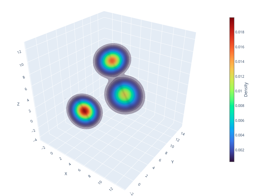

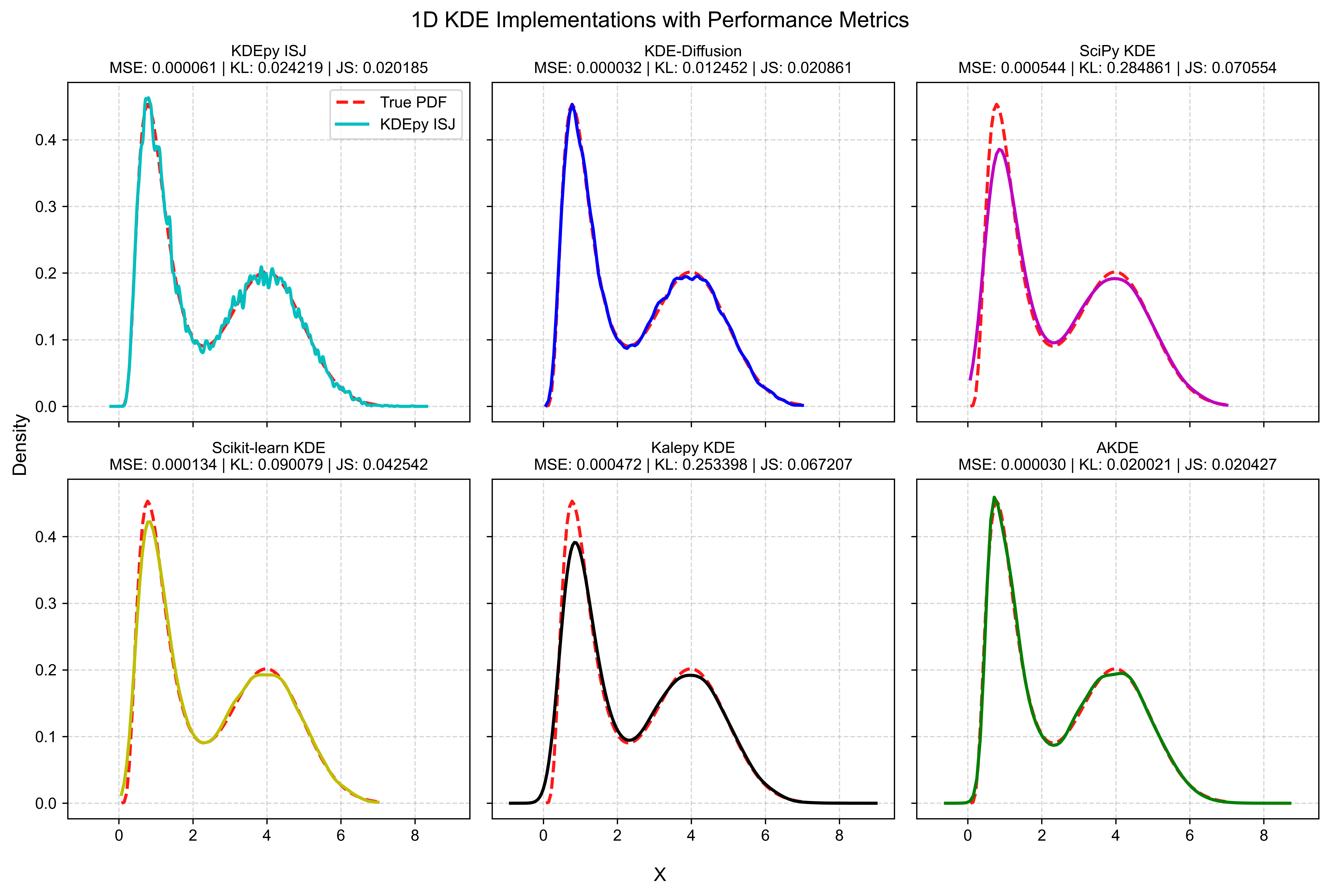
Performance Test

Below, we compare the performance of AKDE with various KDE implementations in Python by computing the Mean Squared Error (MSE), Kullback–Leibler (KL) divergence, and Jensen–Shannon (JS) divergence between the estimated density and the true distribution. Additionally, a goodness-of-fit test can be conducted using the SciPy one-sample or two-sample Kolmogorov-Smirnov test. For multidimensional cases, the fasano.franceschini.test package in R provides an implementation of the multidimensional Kolmogorov-Smirnov two-sample test.

1D KDE implementations with performance metrics

2D KDE implementations with performance metrics

Applications

• Probability density estimation (Galaxy Distribution, Stellar Population, distributions of temperature, wind speed, and precipitation, air pollutant concentration distribution...)
• Anomaly detection (Exoplanet Detection, characterization of rock mass discontinuities...)
• Machine learning preprocessing

License

This project is licensed under the MIT License - see the LICENSE file for details.

Contributions

Contributions are welcome! Feel free to submit a pull request or open an issue.

Author

Trung Nguyen
GitHub: @trungnth
Email: trungnth@dnri.vn

The Math Behind the AKDE

The original MATLAB implementation by Zdravko Botev does not seem to reference the algorithm described in the corresponding paper. Below, we present the mathematical foundation of the algorithm used in the AKDE method.

Kernel density estimation is a widely used statistical tool for estimating the probability density function of data from a finite sample. Traditional KDE techniques estimate the density using a weighted sum of kernel functions centered at the data points. The density is expressed as:

$$ \hat{f}(x) = \frac{1}{n h^d} \sum_{i=1}^n K\left(\frac{x - X_i}{h}\right), $$

where $n$ is the sample size, $h$ is the bandwidth controlling the level of smoothing, $d$ is the dimensionality of the data, and $K$ is the kernel function, commonly chosen as the Gaussian kernel:

$$ K(x) = (2\pi)^{-d/2} \exp\left(-\frac{|x|^2}{2}\right). $$

Despite its utility, traditional KDE suffers from a major challenge: the scaling efficiently to high-dimensional datasets aka The curse of dimensionality. The $\texttt{AKDE}$ method seeks to address these limitations by representing the density as a weighted sum of Gaussian components and refining the parameters of this mixture model iteratively using Expectation-Maximization (EM) algorithm. Unlike classical KDE, which evaluates kernel functions directly for all data points, the $\texttt{AKDE}$ method uses a subset of representative points to approximate the density, significantly reducing computational complexity for high-dimensional data.

Given a dataset $X = {x_1, x_2, \dots, x_n}$ in $\mathbb{R}^d$, Gaussian Mixture Model models the density $f(x)$ of $X$ as a mixture of $K$ Gaussian components, expressed as:

$$ f(x) = \sum_{k=1}^K w_k \phi(x; \mu_k, \Sigma_k), $$

where $w_k$ are non-negative mixture weights satisfying $\sum_{k=1}^K w_k = 1$. The Gaussian components, $\phi(x; \mu_k, \Sigma_k)$, are defined as:

$$ \phi(x; \mu_k, \Sigma_k) = \frac{1}{(2\pi)^{d/2} |\Sigma_k|^{1/2}} \exp\left(-\frac{1}{2}(x - \mu_k)^\top \Sigma_k^{-1} (x - \mu_k)\right). $$

Here, $\mu_k \in \mathbb{R}^d$ and $\Sigma_k \in \mathbb{R}^{d \times d}$ are the mean vector and covariance Hermitian, positive-definite matrix of the $k$-th component and $d$ is the dimensionality of the data. GMMs are particularly well-suited for $\texttt{AKDE}$, as they combine parametric modeling's structure with the flexibility required for adaptive density estimation.

The parameters of the GMM—weights $w_k$, means $\mu_k$, and covariance matrices $\Sigma_k$—are optimized using the EM algorithm, which alternates between the E-step and M-step. The EM algorithm maximizes the log-likelihood of the observed data. For a dataset $X = {x_1, x_2, \dots, x_n}$, the log-likelihood of the GMM is given by:

$$ \mathcal{L}(\Theta; X) = \sum_{i=1}^n \log\left(\sum_{k=1}^K w_k \phi(x_i; \mu_k, \Sigma_k)\right), $$

where $\Theta = {w_k, \mu_k, \Sigma_k}_{k=1}^K$ represents the model parameters.

The algorithm begins by normalizing the input data to fit within a unit hypercube $[0, 1]^d$ for numerical stability. It then initializes $K$ Gaussian components by randomly selecting data points as initial means $\mu_k$. The covariance matrices $\Sigma_k$ are initialized as scaled identity matrices $I$, $\Sigma_k=h^2 \cdot I$ where the scaling $h$ is determined by an initial bandwidth derived from Silverman’s rule of thumb $h = 0.1 / n^{d / (d + 4)}$ and the weights $w_k$ are assigned random values summing to one. These steps ensure a reasonable starting point for optimization.

In the E-step, the algorithm computes the responsibilities $\gamma_{ik}$, which measure the probability that the $k$-th component generated the $i$-th data point $x_i$. This is given by:

$$ \gamma_{ik} = \frac{w_k \phi(x_i; \mu_k, \Sigma_k)}{\sum_{j=1}^K w_j \phi(x_i; \mu_j, \Sigma_j)}. $$

In the M-step, the model parameters are updated using the responsibilities:

$$ w_k = \frac{1}{n} \sum_{i=1}^n \gamma_{ik}, \quad \mu_k = \frac{\sum_{i=1}^n \gamma_{ik} x_i}{\sum_{i=1}^n \gamma_{ik}}, \quad \Sigma_k = \frac{\sum_{i=1}^n \gamma_{ik} (x_i - \mu_k)(x_i - \mu_k)^\top}{\sum_{i=1}^n \gamma_{ik}}. $$

These updates ensure that the log-likelihood of the data increases with each iteration. The EM process is implemented in the regEM function in AKDE, which terminates when the change in log-likelihood is below a predefined tolerance.

After optimizing the GMM parameters, the algorithm evaluates the estimated density function $f(x)$ over a grid of points to enable visualization. This evaluation requires efficient computation of the Gaussian components for large datasets, which is achieved using Cholesky decomposition to factorize each covariance matrix $\Sigma_k$ as:

$$ \Sigma_k = L_k L_k^\top, $$

where $L_k$ is a lower triangular matrix. This decomposition simplifies several key operations:

$$ |\Sigma_k| = \prod_{i=1}^d (L_k[i, i])^2, $$

$$ \Sigma_k^{-1} = (L_k^\top)^{-1} L_k^{-1}, $$

$$ (x - \mu_k)^\top \Sigma_k^{-1} (x - \mu_k) = |L_k^{-1} (x - \mu_k)|^2. $$

These computations, implemented in the probfun function, are critical for the efficient and stable evaluation of the GMM.

A unique feature of AKDE is the dynamic adjustment of bandwidths for each Gaussian component based on the local curvature of the density. The curvature $\text{curv}$ is defined as:

$$ \text{curv} = \int |\nabla^2 f(x)|_F^2 f(x) , dx, $$

where $|\nabla^2 f(x)|_F^2$ is the squared Frobenius norm of the Hessian matrix $\nabla^2 f(x)$, given by:

$$ |\nabla^2 f(x)|_F^2 = \sum_{i=1}^d \sum_{j=1}^d \left(\frac{\partial^2 f(x)}{\partial x_i \partial x_j}\right)^2. $$

The bandwidth $h_k$ for each component is then computed as:

$$ h_k = \left(\frac{1}{4n \pi^{d/2} |I|^{1/2} \cdot \text{curv}}\right)^{1/(d+2)}, $$

where $n$ is the number of data points, $d$ is the dimensionality, and $I$ is the identity matrix. Smaller bandwidths are assigned to regions of high curvature, improving the local adaptivity of the density estimate.

Entropy is used as a criterion to ensure the smoothness and generality of the density estimate. The entropy of the estimated density $f(x)$ is defined as:

$$ H = -\int f(x) \log f(x) , dx. $$

The algorithm maximizes entropy iteratively, promoting a smooth and unbiased density estimate while avoiding overfitting. The AKDE implementation demonstrates the power of Gaussian Mixture Models in adaptive kernel density estimation. By combining the EM algorithm for parameter optimization, curvature-based bandwidth selection, and entropy maximization, the algorithm achieves flexible and accurate density estimation. The use of Cholesky decomposition ensures computational efficiency and stability, making the algorithm scalable for large datasets and high-dimensional problems. This seamless integration of mathematical rigor and computational efficiency highlights the versatility of GMMs in density estimation.